Expression Tree Construction

A binary expression tree is a specific kind of a binary tree used to represent expressions

The leaves of a binary expression tree are operands, such as constants or variable names, and the other nodes contain operators. These particular trees happen to be binary, because all of the operations are binary, and although this is the simplest case, it is possible for nodes to have more than two children. It is also possible for a node to have only one child, as is the case with the unary minus operator

Construction of an expression tree

The evaluation of the tree takes place by reading the postfix expression one symbol at a time. If the symbol is an operand, one-node tree is created and a pointer is pushed onto a stack. If the symbol is an operator, the pointers are popped to two trees T1 and T2 from the stack and a new tree whose root is the operator and whose left and right children point to T2 and T1 respectively is formed . A pointer to this new tree is then pushed to the Stack

Example

The input is: a b + c d e + * * Since the first two symbols are operands, one-node trees are created and pointers are pushed to them onto a stack. For convenience the stack will grow from left to right.

Stack growing from left to right

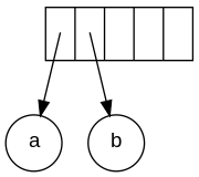
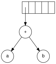
The next symbol is a '+'. It pops the two pointers to the trees, a new tree is formed, and a pointer to it is pushed onto to the stack.

Formation of a new tree

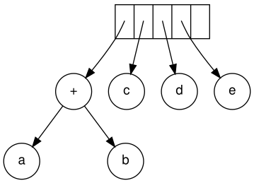
Next, c, d, and e are read. A one-node tree is created for each and a pointer to the corresponding tree is pushed onto the stack.

Creating a one-node tree

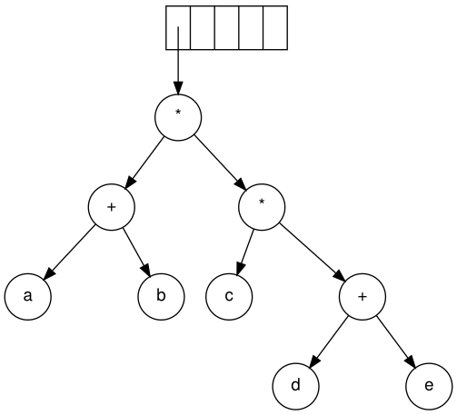
Continuing, a '+' is read, and it merges the last two trees.

Merging two trees

Now, a '*' is read. The last two tree pointers are popped and a new tree is formed with a '*' as the root.

Forming a new tree with a root

Finally, the last symbol is read. The two trees are merged and a pointer to the final tree remains on the stack.^[5]

Steps to construct an expression tree a b + c d e + * *

 

Postfix Expression Evaluation

A postfix expression is a collection of operators and operands in which the operator is placed after the operands. That means, in a postfix expression the operator follows the operands.

Postfix Expression has following general structure...

Operand1 Operand2 Operator

Example

Postfix Expression Evaluation using Stack Data Structure

A postfix expression can be evaluated using the Stack data structure. To evaluate a postfix expression using Stack data structure we can use the following steps...

Read all the symbols one by one from left to right in the given Postfix Expression

If the reading symbol is operand, then push it on to the Stack.

If the reading symbol is operator (+ , - , * , / etc.,), then perform TWO pop operations and store the two popped oparands in two different variables (operand1 and operand2). Then perform reading symbol operation using operand1 and operand2 and push result back on to the Stack.

Finally! perform a pop operation and display the popped value as final result.

Example

Consider the following Expression...

Expressions

What is an Expression?

In any programming language, if we want to perform any calculation or to frame a condition etc., we use a set of symbols to perform the task. These set of symbols makes an expression.

An expression can be defined as follows...

An expression is a collection of operators and operands that represents a specific value.

In above definition, operator is a symbol which performs a particular task like arithmetic operation or logical operation or conditional operation etc.,

Operands are the values on which the operators can perform the task. Here operand can be a direct value or variable or address of memory location.

Expression Types

Based on the operator position, expressions are divided into THREE types. They are as follows...

Infix Expression

Postfix Expression

Prefix Expression

Infix Expression

In infix expression, operator is used in between operands.

The general structure of an Infix expression is as follows...

Operand1 Operator Operand2

Example

Postfix Expression

In postfix expression, operator is used after operands. We can say that "Operator follows the Operands".

The general structure of Postfix expression is as follows...

Operand1 Operand2 Operator

Example

Prefix Expression

In prefix expression, operator is used before operands. We can say that "Operands follows the Operator".

The general structure of Prefix expression is as follows...

Operator Operand1 Operand2

Example

Any expression can be represented using the above three different types of expressions. And we can convert an expression from one form to another form like Infix to Postfix, Infix to Prefix, Prefix to Postfix and vice versa.

Binary Tree Traversals

When we wanted to display a binary tree, we need to follow some order in which all the nodes of that binary tree must be displayed. In any binary tree displaying order of nodes depends on the traversal method.

Displaying (or) visiting order of nodes in a binary tree is called as Binary Tree Traversal.

There are three types of binary tree traversals.

1. In - Order Traversal
2. Pre - Order Traversal
3. Post - Order Traversal

Consider the following binary tree...

 

1. In - Order Traversal ( leftChild - root - rightChild )

In In-Order traversal, the root node is visited between left child and right child. In this traversal, the left child node is visited first, then the root node is visited and later we go for visiting right child node. This in-order traversal is applicable for every root node of all subtrees in the tree. This is performed recursively for all nodes in the tree.

In the above example of binary tree, first we try to visit left child of root node 'A', but A's left child is a root node for left subtree. so we try to visit its (B's) left child 'D' and again D is a root for subtree with nodes D, I and J. So we try to visit its left child 'I' and it is the left most child. So first we visit 'I' then go for its root node 'D' and later we visit D's right child 'J'. With this we have completed the left part of node B. Then visit 'B' and next B's right child 'F' is visited. With this we have completed left part of node A. Then visit root node 'A'. With this we have completed left and root parts of node A. Then we go for right part of the node A. In right of A again there is a subtree with root C. So go for left child of C and again it is a subtree with root G. But G does not have left part so we visit 'G' and then visit G's right child K. With this we have completed the left part of node C. Then visit root node 'C' and next visit C's right child 'H' which is the right most child in the tree so we stop the process.

That means here we have visited in the order of I - D - J - B - F - A - G - K - C - H using In-Order Traversal.

In-Order Traversal for above example of binary tree is

I - D - J - B - F - A - G - K - C - H

 

2. Pre - Order Traversal ( root - leftChild - rightChild )

In Pre-Order traversal, the root node is visited before left child and right child nodes. In this traversal, the root node is visited first, then its left child and later its right child. This pre-order traversal is applicable for every root node of all subtrees in the tree.

In the above example of binary tree, first we visit root node 'A' then visit its left child 'B' which is a root for D and F. So we visit B's left child 'D' and again D is a root for I and J. So we visit D's left child 'I' which is the left most child. So next we go for visiting D's right child 'J'. With this we have completed root, left and right parts of node D and root, left parts of node B. Next visit B's right child 'F'. With this we have completed root and left parts of node A. So we go for A's right child 'C' which is a root node for G and H. After visiting C, we go for its left child 'G' which is a root for node K. So next we visit left of G, but it does not have left child so we go for G's right child 'K'. With this we have completed node C's root and left parts. Next visit C's right child 'H' which is the right most child in the tree. So we stop the process.

That means here we have visited in the order of A-B-D-I-J-F-C-G-K-H using Pre-Order Traversal.

Pre-Order Traversal for above example binary tree is

A - B - D - I - J - F - C - G - K - H

 

3. Post - Order Traversal ( leftChild - rightChild - root )

In Post-Order traversal, the root node is visited after left child and right child. In this traversal, left child node is visited first, then its right child and then its root node. This is recursively performed until the right most node is visited.

Here we have visited in the order of I - J - D - F - B - K - G - H - C - A using Post-Order Traversal.

Post-Order Traversal for above example binary tree is

I - J - D - F - B - K - G - H - C - A

Program to Create Binary Tree and display using In-Order Traversal.

#include
#include

struct Node{
   int data;
   struct Node *left;
   struct Node *right;
};

struct Node *root = NULL;
int count = 0;

struct Node* insert(struct Node*, int);
void display(struct Node*);

void main(){
   int choice, value;
   clrscr();
   printf("\n----- Binary Tree -----\n");
   while(1){
      printf("\n***** MENU *****\n");
      printf("1. Insert\n2. Display\n3. Exit");
      printf("\nEnter your choice: ");
      scanf("%d",&choice);
      switch(choice){
  case 1: printf("\nEnter the value to be insert: ");
   scanf("%d", &value);
   root = insert(root,value);
   break;
  case 2: display(root); break;
  case 3: exit(0);
  default: printf("\nPlease select correct operations!!!\n");
      }
   }
}

struct Node* insert(struct Node *root,int value){
   struct Node *newNode;
   newNode = (struct Node*)malloc(sizeof(struct Node));
   newNode->data = value;
   if(root == NULL){
      newNode->left = newNode->right = NULL;
      root = newNode;
      count++;
   }
   else{
      if(count%2 != 0)
  root->left = insert(root->left,value);
      else
  root->right = insert(root->right,value);
   }
   return root;
}
// display is performed by using Inorder Traversal
void display(struct Node *root)
{
   if(root != NULL){
      display(root->left);
      printf("%d\t",root->data);
      display(root->right);
   }
}

Output

 

Binary Tree

In a normal tree, every node can have any number of children. Binary tree is a special type of tree data structure in which every node can have a maximum of 2 children. One is known as left child and the other is known as right child.

A tree in which every node can have a maximum of two children is called as Binary Tree.

In a binary tree, every node can have either 0 children or 1 child or 2 children but not more than 2 children.

Example

There are different types of binary trees and they are...

1. Strictly Binary Tree

In a binary tree, every node can have a maximum of two children. But in strictly binary tree, every node should have exactly two children or none. That means every internal node must have exactly two children. A strictly Binary Tree can be defined as follows...

A binary tree in which every node has either two or zero number of children is called Strictly Binary Tree

---

Strictly binary tree is also called as Full Binary Tree or Proper Binary Tree or 2-Tree

---

Strictly binary tree data structure is used to represent mathematical expressions.

Example

2. Complete Binary Tree

In a binary tree, every node can have a maximum of two children. But in strictly binary tree, every node should have exactly two children or none and in complete binary tree all the nodes must have exactly two children and at every level of complete binary tree there must be 2^level number of nodes. For example at level 2 there must be 2² = 4 nodes and at level 3 there must be 2³ = 8 nodes.

A binary tree in which every internal node has exactly two children and all leaf nodes are at same level is called Complete Binary Tree.

---

Complete binary tree is also called as Perfect Binary Tree

---

3. Extended Binary Tree

A binary tree can be converted into Full Binary tree by adding dummy nodes to existing nodes wherever required.

The full binary tree obtained by adding dummy nodes to a binary tree is called as Extended Binary Tree.

In above figure, a normal binary tree is converted into full binary tree by adding dummy nodes (In pink colour).

Application of a Binary Tree

The binary tree are applicable in the below mentioned fields:
- Used in the compilers of high-level programming languages for intermediate representation
- Used as a searching technique
- Used in databases for storing data
- To solve arithmetic expressions

Tree Representations

A tree data structure can be represented in two methods. Those methods are as follows...

1. List Representation
2. Left Child - Right Sibling Representation

Consider the following tree...

1. List Representation

In this representation, we use two types of nodes one for representing the node with data and another for representing only references. We start with a node with data from root node in the tree. Then it is linked to an internal node through a reference node and is linked to any other node directly. This process repeats for all the nodes in the tree.

The above tree example can be represented using List representation as follows...

2. Left Child - Right Sibling Representation

In this representation, we use list with one type of node which consists of three fields namely Data field, Left child reference field and Right sibling reference field. Data field stores the actual value of a node, left reference field stores the address of the left child and right reference field stores the address of the right sibling node. Graphical representation of that node is as follows...

In this representation, every node's data field stores the actual value of that node. If that node has left child, then left reference field stores the address of that left child node otherwise that field stores NULL. If that node has right sibling then right reference field stores the address of right sibling node otherwise that field stores NULL.

The above tree example can be represented using Left Child - Right Sibling representation as follows...

Tree Terminology

In linear data structure, data is organized in sequential order and in non-linear data structure, data is organized in random order. Tree is a very popular data structure used in wide range of applications.

A tree data structure can be defined as follows...

       Tree is a non-linear data structure which organizes data in hierarchical structure and this is a recursive definition.

A tree data structure can also be defined as follows...

      Tree data structure is a collection of data (Node) which is organized in hierarchical structure and this is a recursive definition

In tree data structure, every individual element is called as Node. Node in a tree data structure, stores the actual data of that particular element and link to next element in hierarchical structure.

In a tree data structure, if we have N number of nodes then we can have a maximum of N-1 number of links.

Example

Terminology

In a tree data structure, we use the following terminology...

1. Root

In a tree data structure, the first node is called as Root Node. Every tree must have root node. We can say that root node is the origin of tree data structure. In any tree, there must be only one root node. We never have multiple root nodes in a tree.

2. Edge

In a tree data structure, the connecting link between any two nodes is called as EDGE. In a tree with 'N' number of nodes there will be a maximum of 'N-1' number of edges.

3. Parent

In a tree data structure, the node which is predecessor of any node is called as PARENT NODE. In simple words, the node which has branch from it to any other node is called as parent node. Parent node can also be defined as "The node which has child / children".

4. Child

In a tree data structure, the node which is descendant of any node is called as CHILD Node. In simple words, the node which has a link from its parent node is called as child node. In a tree, any parent node can have any number of child nodes. In a tree, all the nodes except root are child nodes.

5. Siblings

In a tree data structure, nodes which belong to same Parent are called as SIBLINGS. In simple words, the nodes with same parent are called as Sibling nodes.

6. Leaf

In a tree data structure, the node which does not have a child is called as LEAF Node. In simple words, a leaf is a node with no child.

In a tree data structure, the leaf nodes are also called as External Nodes. External node is also a node with no child. In a tree, leaf node is also called as 'Terminal' node.

7. Internal Nodes

In a tree data structure, the node which has atleast one child is called as INTERNAL Node. In simple words, an internal node is a node with atleast one child.

In a tree data structure, nodes other than leaf nodes are called as Internal Nodes. The root node is also said to be Internal Node if the tree has more than one node. Internal nodes are also called as 'Non-Terminal' nodes.

8. Degree

In a tree data structure, the total number of children of a node is called as DEGREE of that Node. In simple words, the Degree of a node is total number of children it has. The highest degree of a node among all the nodes in a tree is called as 'Degree of Tree'

9. Level

In a tree data structure, the root node is said to be at Level 0 and the children of root node are at Level 1 and the children of the nodes which are at Level 1 will be at Level 2 and so on... In simple words, in a tree each step from top to bottom is called as a Level and the Level count starts with '0' and incremented by one at each level (Step).

10. Height

In a tree data structure, the total number of egdes from leaf node to a particular node in the longest path is called as HEIGHT of that Node. In a tree, height of the root node is said to be height of the tree. In a tree, height of all leaf nodes is '0'.

11. Depth

In a tree data structure, the total number of egdes from root node to a particular node is called as DEPTH of that Node. In a tree, the total number of edges from root node to a leaf node in the longest path is said to be Depth of the tree. In simple words, the highest depth of any leaf node in a tree is said to be depth of that tree. In a tree, depth of the root node is '0'.

12. Path

In a tree data structure, the sequence of Nodes and Edges from one node to another node is called as PATH between that two Nodes. Length of a Path is total number of nodes in that path. In below example the path A - B - E - J has length 4.

13. Sub Tree

In a tree data structure, each child from a node forms a subtree recursively. Every child node will form a subtree on its parent node.

---

Animations

Non Linear Data Structures

What is a non-linear datastructure?

A non-linear data structure is a data structure in which a data item is connected to several other data items. So that a given data item has the possibility to reach one-or-more data items.

Pros

• Uses memory efficiently that the free contiguous memory in not an requirement for allocating data items
• The length of the data items is not necessary to be known prior to allocation

Cons

• Overhead of the link to the next data item

Examples of non-linear data-structures are Graphs and Trees. However Linked List and Arrays are linear data structures.

Introduction to Data Structures

What is Data Structure?

Whenever we want to work with large amount of data, then organizing that data is very important. If that data is not organized effectively, it is very difficult to perform any task on that data. If it is organized effectively then any operation can be performed easily on that data.

A data structure can be defined as follows...

Data structure is a method of organizing large amount of data more efficiently so that any operation on that data becomes easy

NOTE

• Every data structure is used to organize the large amount of data
• Every data structure follows a particular principle
• The operations in a data structure should not violate the basic principle of that data structure.

Based on the organizing method of a data structure, data structures are divided into two types.

1. Linear Data Structures
2. Non - Linear Data Structures

Linear Data Structures

If a data structure is organizing the data in sequential order, then that data structure is called as Linear Data Structure.

Example

1. Arrays
2. List (Linked List)
3. Stack
4. Queue

Non - Linear Data Structures

If a data structure is organizing the data in random order, then that data structure is called as Non-Linear Data Structure.

Example

1. Tree
2. Graph
3. Dictionaries
4. Heaps
5. Tries, Etc.,

Asymptotic Notation

What is Asymptotic Notation?

Whenever we want to perform analysis of an algorithm, we need to calculate the complexity of that algorithm. But when we calculate complexity of an algorithm it does not provide exact amount of resource required. So instead of taking exact amount of resource we represent that complexity in a general form (Notation) which produces the basic nature of that algorithm. We use that general from (Notation) for analysis process.

Asymptotic notation of an algorithm is a mathematical representation of its complexity

NOTE

☀ In asymptotic notation, when we want to represent the complexity of an algorithm, we use only the most significant terms in the complexity of that algorithm and ignore least significant terms in the complexity of that algorithm (Here complexity may be Space Complexity or Time Complexity).

For example, consider the following time complexities of two algorithms...

• Algorihtm 1 : 5n² + 2n + 1
• Algorihtm 2 : 10n² + 8n + 3

Generally, when we analyze an algorithm, we consider the time complexity for larger values of input data (i.e. 'n' value). In above two time complexities, for larger value of 'n' the term in algorithm 1 '2n + 1' has least significance than the term '5n²', and the term in algorithm 2 '8n + 3' has least significance than the term '10n²'.

Here for larger value of 'n' the value of most significant terms ( 5n² and 10n² ) is very larger than the value of least significant terms ( 2n + 1 and 8n + 3 ). So for larger value of 'n' we ignore the least significant terms to represent overall time required by an algorithm. In asymptotic notation, we use only the most significant terms to represent the time complexity of an algorithm.

Majorly, we use THREE types of Asymptotic Notations and those are as follows...

1. Big - Oh (O)
2. Big - Omega (Ω)
3. Big - Theta (Θ)

Big - Oh Notation (O)

Big - Oh notation is used to define the upper bound of an algorithm in terms of Time Complexity.

That means Big - Oh notation always indicates the maximum time required by an algorithm for all input values. That means Big - Oh notation describes the worst case of an algorithm time complexity.

Big - Oh Notation can be defined as follows...

Consider function f(n) the time complexity of an algorithm and g(n) is the most significant term. If f(n) <= C g(n) for all n >= n₀, C > 0 and n₀ >= 1. Then we can represent f(n) as O(g(n)).

f(n) = O(g(n))

Consider the following graph drawn for the values of f(n) and C g(n) for input (n) value on X-Axis and time required is on Y-Axis

In above graph after a particular input value n₀, always C g(n) is greater than f(n) which indicates the algorithm's upper bound.

Example

Consider the following f(n) and g(n)...
f(n) = 3n + 2
g(n) = n
If we want to represent f(n) as O(g(n)) then it must satisfy f(n) <= C x g(n) for all values of C > 0 and n₀>= 1

f(n) <= C g(n)
⇒3n + 2 <= C n

Above condition is always TRUE for all values of C = 4 and n >= 2.
By using Big - Oh notation we can represent the time complexity as follows...
3n + 2 = O(n)

Big - Omege Notation (Ω)

Big - Omega notation is used to define the lower bound of an algorithm in terms of Time Complexity.

That means Big - Omega notation always indicates the minimum time required by an algorithm for all input values. That means Big - Omega notation describes the best case of an algorithm time complexity.

Big - Omega Notation can be defined as follows...

Consider function f(n) the time complexity of an algorithm and g(n) is the most significant term. If f(n) >= C x g(n) for all n >= n₀, C > 0 and n₀ >= 1. Then we can represent f(n) as Ω(g(n)).

f(n) = Ω(g(n))

Consider the following graph drawn for the values of f(n) and C g(n) for input (n) value on X-Axis and time required is on Y-Axis

In above graph after a particular input value n₀, always C x g(n) is less than f(n) which indicates the algorithm's lower bound.

Example

Consider the following f(n) and g(n)...
f(n) = 3n + 2
g(n) = n
If we want to represent f(n) as Ω(g(n)) then it must satisfy f(n) >= C g(n) for all values of C > 0 and n₀>= 1

f(n) >= C g(n)
⇒3n + 2 <= C n

Above condition is always TRUE for all values of C = 1 and n >= 1.
By using Big - Omega notation we can represent the time complexity as follows...
3n + 2 = Ω(n)

Big - Theta Notation (Θ)

Big - Theta notation is used to define the average bound of an algorithm in terms of Time Complexity.

That means Big - Theta notation always indicates the average time required by an algorithm for all input values. That means Big - Theta notation describes the average case of an algorithm time complexity.

Big - Theta Notation can be defined as follows...

Consider function f(n) the time complexity of an algorithm and g(n) is the most significant term. If C₁ g(n) <= f(n) >= C₂ g(n) for all n >= n₀, C₁, C₂ > 0 and n₀ >= 1. Then we can represent f(n) as Θ(g(n)).

f(n) = Θ(g(n))

Consider the following graph drawn for the values of f(n) and C g(n) for input (n) value on X-Axis and time required is on Y-Axis

In above graph after a particular input value n₀, always C₁ g(n) is less than f(n) and C₂ g(n) is greater than f(n) which indicates the algorithm's average bound.

Example

Consider the following f(n) and g(n)...
f(n) = 3n + 2
g(n) = n
If we want to represent f(n) as Θ(g(n)) then it must satisfy C₁ g(n) <= f(n) >= C₂ g(n) for all values of C₁, C₂ > 0 and n₀>= 1

C₁ g(n) <= f(n) >= ⇒C₂ g(n)
C₁ n <= 3n + 2 >= C₂ n

Above condition is always TRUE for all values of C₁ = 1, C₂ = 4 and n >= 1.
By using Big - Theta notation we can represent the time compexity as follows...
3n + 2 = Θ(n)

Time Complexity

What is Time complexity?

Every algorithm requires some amount of computer time to execute its instruction to perform the task. This computer time required is called time complexity.

Time complexity of an algorithm can be defined as follows...

The time complexity of an algorithm is the total amount of time required by an algorithm to complete its execution.

Generally, running time of an algorithm depends upon the following...

1. Whether it is running on Single processor machine or Multi processor machine.
2. Whether it is a 32 bit machine or 64 bit machine
3. Read and Write speed of the machine.
4. The time it takes to perform Arithmetic operations, logical operations, return value and assignment operations etc.,
5. Input data

NOTE

☀ When we calculate time complexity of an algorithm, we consider only input data and ignore the remaining things, as they are machine dependent. We check only, how our program is behaving for the different input values to perform all the operations like Arithmetic, Logical, Return value and Assignment etc.,

Calculating Time Complexity of an algorithm based on the system configuration is a very difficult task because, the configuration changes from one system to another system. To solve this problem, we must assume a model machine with specific configuration. So that, we can able to calculate generalized time complexity according to that model machine.

To calculate time complexity of an algorithm, we need to define a model machine. Let us assume a machine with following configuration...

1. Single processor machine
2. 32 bit Operating System machine
3. It performs sequential execution
4. It requires 1 unit of time for Arithmetic and Logical operations
5. It requires 1 unit of time for Assignment and Return value
6. It requires 1 unit of time for Read and Write operations

Now, we calculate the time complexity of following example code by using the above defined model machine...

Example 1

Consider the following piece of code...

int sum(int a, int b)
{
   return a+b;
}

In above sample code, it requires 1 unit of time to calculate a+b and 1 unit of time to return the value. That means, totally it takes 2 units of time to complete its execution. And it does not change based on the input values of a and b. That means for all input values, it requires same amount of time i.e. 2 units.

If any program requires fixed amount of time for all input values then its time complexity is said to be Constant Time Complexity.

Example 2

Consider the following piece of code...

int sum(int A[], int n)
{
   int sum = 0, i;
   for(i = 0; i < n; i++)
      sum = sum + A[i];
   return sum;
}

For the above code, time complexity can be calculated as follows...

In above calculation
Cost is the amount of computer time required for a single operation in each line.
Repeatation is the amount of computer time required by each operation for all its repeatations.
Total is the amount of computer time required by each operation to execute.

So above code requires '4n+4' Units of computer time to complete the task. Here the exact time is not fixed. And it changes based on the n value. If we increase the n value then the time required also increases linearly.

Totally it takes '4n+4' units of time to complete its execution and it is Linear Time Complexity.

If the amount of time required by an algorithm is increased with the increase of input value then that time complexity is said to be Linear Time Complexity

Space Complexity

What is Space complexity?

When we design an algorithm to solve a problem, it needs some computer memory to complete its execution. For any algorithm, memory is required for the following purposes...

1. Memory required to store program instructions
2. Memory required to store constant values
3. Memory required to store variable values
4. And for few other things

Space complexity of an algorithm can be defined as follows...

Total amount of computer memory required by an algorithm to complete its execution is called as space complexity of that algorithm

Generally, when a program is under execution it uses the computer memory for THREE reasons. They are as follows...

1. Instruction Space: It is the amount of memory used to store compiled version of instructions.
2. Environmental Stack: It is the amount of memory used to store information of partially executed functions at the time of function call.
3. Data Space: It is the amount of memory used to store all the variables and constants.

NOTE

☀ When we want to perform analysis of an algorithm based on its Space complexity, we consider only Data Space and ignore Instruction Space as well as Environmental Stack.
That means we calculate only the memory required to store Variables, Constants, Structures, etc.,

To calculate the space complexity, we must know the memory required to store different datatype values (according to the compiler). For example, the C Programming Language compiler requires the following...

1. 2 bytes to store Integer value,
2. 4 bytes to store Floating Point value,
3. 1 byte to store Character value,
4. 6 (OR) 8 bytes to store double value

Example 1

Consider the following piece of code...

int square(int a)
{
 return a*a;
}

In above piece of code, it requires 2 bytes of memory to store variable 'a' and another 2 bytes of memory is used for return value.

That means, totally it requires 4 bytes of memory to complete its execution. And this 4 bytes of memory is fixed for any input value of 'a'. This space complexity is said to be Constant Space Complexity.

If any algorithm requires a fixed amount of space for all input values then that space complexity is said to be Constant Space Complexity

Example 2

Consider the following piece of code...

int sum(int A[], int n)
{
   int sum = 0, i;
   for(i = 0; i < n; i++)
      sum = sum + A[i];
   return sum;
}

In above piece of code it requires

'n*2' bytes of memory to store array variable 'a[]'
2 bytes of memory for integer parameter 'n'
4 bytes of memory for local integer variables 'sum' and 'i' (2 bytes each)
2 bytes of memory for return value.

That means, totally it requires '2n+8' bytes of memory to complete its execution. Here, the amount of memory depends on the input value of 'n'. This space complexity is said to be Linear Space Complexity.

If the amount of space required by an algorithm is increased with the increase of input value, then that space complexity is said to be Linear Space Complexity

Performance Analysis

What is Performance Analysis of an algorithm?

If we want to go from city "A" to city "B", there can be many ways of doing this. We can go by flight, by bus, by train and also by bicycle. Depending on the availability and convenience, we choose the one which suits us. Similarly, in computer science there are multiple algorithms to solve a problem. When we have more than one algorithm to solve a problem, we need to select the best one. Performance analysis helps us to select the best algorithm from multiple algorithms to solve a problem.

When there are multiple alternative algorithms to solve a problem, we analyse them and pick the one which is best suitable for our requirements. Formal definition is as follows...

Performance of an algorithm is a process of making evaluative judgement about algorithms.

It can also be defined as follows...

Performance of an algorithm means predicting the resources which are required to an algorithm to perform its task.

That means when we have multiple algorithms to solve a problem, we need to select a suitable algorithm to solve that problem.

We compare all algorithms with each other which are solving same problem, to select best algorithm. To compare algorithms, we use a set of parameters or set of elements like memory required by that algorithm, execution speed of that algorithm, easy to understand, easy to implement, etc.,

Generally, the performance of an algorithm depends on the following elements...

1. Whether that algorithm is providing the exact solution for the problem?
2. Whether it is easy to understand?
3. Whether it is easy to implement?
4. How much space (memory) it requires to solve the problem?
5. How much time it takes to solve the problem? Etc.,

When we want to analyse an algorithm, we consider only the space and time required by that particular algorithm and we ignore all remaining elements.

Based on this information, performance analysis of an algorithm can also be defined as follows...

Performance analysis of an algorithm is the process of calculating space required by that algorithm and time required by that algorithm.

Performance analysis of an algorithm is performed by using the following measures...

1. Space required to complete the task of that algorithm (Space Complexity). It includes program space and data space
2. Time required to complete the task of that algorithm (Time Complexity)

Introduction to Algorithm

An algorithm is a step by step procedure to solve a problem. In normal language, algorithm is defined as a sequence of statements which are used to perform a task. In computer science, an algorithm can be defined as follows...

An algorithm is a sequence of unambiguous instructions used for solving a problem, which can be implemented (as a program) on a computer

Algorithms are used to convert our problem solution into step by step statements. These statements can be converted into computer programming instructions which forms a program. This program is executed by computer to produce solution. Here, program takes required data as input, processes data according to the program instructions and finally produces result as shown in the following picture.

Algorithm Specifications

Every algorithm must satisfy the following specifications...

1. Input - Every algorithm must take zero or more number of input values from external.
2. Output - Every algorithm must produce an output as result.
3. Definiteness - Every statement/instruction in an algorithm must be clear and unambiguous (only one interpretation)
4. Finiteness - For all different cases, the algorithm must produce result within a finite number of steps.
5. Effectiveness - Every instruction must be basic enough to be carried out and it also must be feasible.

Example of Algorithm

Let us consider the following problem for finding the largest value in a given list of values.

Problem Statement : Find the largest number in the given list of numbers?
Input : A list of positive integer numbers. (List must contain at least one number).
Output : The largest number in the given list of positive integer numbers.

Consider the given list of numbers as 'L' (input), and the largest number as 'max' (Output).

Algorithm

• Step 1: Define a variable 'max' and initialize with '0'.
• Step 2: Compare first number (say 'x') in the list 'L' with 'max', if 'x' is larger than 'max', set 'max' to 'x'.
• Step 3: Repeat step 2 for all numbers in the list 'L'.
• Step 4: Display the value of 'max' as a result.

Code in C Programming

int findMax(L)
{
   int max = 0,i;
   for(i=0; i < listSize; i++)
   {
      if(L[i] > max)
         max = L[i];
   }
   return max;
}

Recursive Algorithm

In computer science, all algorithms are implemented with programming language functions. We can view a function as something that is invoked (called) by another function. It executes its code and then returns control to the calling function. Here, a function can call themselves (by itself) or it may call another function which again call same function inside it.

The function which calls by itself is called as Direct Recursive function (or Recursive function)

A recursive algorithm can also be defined as follows...

The function which calls a function and that function calls its called function is called Indirect Recursive function (or Recursive function)

Most of the computer science students think that recursive is a technique useful for only a few special problems like computing factorials, Ackermann's function etc., This is unfortunate because any function implemented using assignment or if-else or while or looping statements can also be implemented using recursive functions. This recursive function is very easier to understand when compared to its iterative counterpart.

Welcome!!

Hi guys, i am happy to welcome to my blog on Advanced data structures. This blog will have all the resources that you will need to learn data structures easily. All the very BEST :)